statistics

1.期望

李航统计与机器学习书中理论模型中的风险函数 (risk function)定义如下，代表一种理想情况下计算误差代价的方法。

​ $R{exp}(f) = E[Y, L(X)] = \sum{X,Y}L(y, f(x))P(x, y) = \int_{X,Y}L(y,f(x))P(x,y)dxdy$

而在4.1.2 章后验概率最大化的地方有个公式：

​ $R{exp}(f) = E_x \sum{i=1}^K[L(c_k, f(X))]P(c_k|X)$

初看比较费解，怎么变成条件概率了？

其实这个公式要从多重积分的角度考虑就明显了，相当于：

​ $\int_X[\int_Y f(x,y)p(x,y)dy]dx$.

在对$y$积分的时候，$x$相当于一个常量，从这一角度考虑，正好就是 $p(y|x)$ ，即一个条件概率形式。

2.Estimator 估计量

a function of the data that is used to infer the value of an unknown parameter in a statistical model,can be writed like $\hat{\theta}(X)$.”估计量”是样本空间映射到样本估计值的一个函数 (Then an estimator is a function that maps the sample space to a set of sample estimates.)估计量用来估计未知总体的参数，它有时也被称为估计子；一次估计是指把这个函数应用在一组已知的数据集上，求函数的结果。对于给定的参数，可以有许多不同的估计量。

Estimand

The parameter being estimated,like $\theta$.
Estimate: a particular realization of this random variable $\hat{\theta}(X)$ is called the “estimate”,like $\hat{\theta}(x)$.

Bias: The bias of $\widehat{\theta}$ is defined as $B(\widehat{ \theta }) = \operatorname{ E }(\widehat{ \theta }) - \theta$.
It is the distance between the average of the collection of estimates, and the single parameter being estimated. It also is the expected value of the error, since

$$\operatorname{E}(\widehat{\theta}) - \theta = \operatorname{E}(\widehat{ \theta } - \theta)$$

The estimator $\widehat{\theta}$ is an unbiased estimator of $\theta$ if and only if $B(\widehat{ \theta }) = 0$.example: If the parameter is the bull’s-eye of a target, and the arrows are estimates, then a relatively high absolute value for the bias means the average position of the arrows is off-target, and a relatively low absolute bias means the average position of the arrows is on target. They may be dispersed, or may be clustered.

Variance(方差)

The variance of $\widehat{\theta}$ is simply the expected value of the squared sampling deviations; that is, $\operatorname{var}(\widehat{ \theta }) = \operatorname{E}[(\widehat{ \theta } - \operatorname{E}(\widehat{\theta}) )^2]$. It is used to indicate how far, on average, the collection of estimates are from the expected value(期望) of the estimates.

example

If the parameter is the bull’s-eye of a target, and the arrows are estimates, then a relatively high variance means the arrows are dispersed, and a relatively low variance means the arrows are clustered. Some things to note: even if the variance is low, the cluster of arrows may still be far off-target, and even if the variance is high, the diffuse collection of arrows may still be unbiased. Finally, note that even if all arrows grossly miss the target, if they nevertheless all hit the same point, the variance is zero.
The relationship between bias and variance is analogous to the relationship between accuracy and precision.

note:the sample mean ${\overline{X}}=\frac{1}{N}\sum_{i=1}^{N}{X}_i$ is an unbiased estimator of $μ$,and the sample variance

$s^2=\frac{1}{n-1}\sum{i=1}^n(X_i-\overline{X}\,)^2$ is an unbiased estimator of $σ^2$,(not the
$S^2=\frac{1}{n}\sum{i=1}^n\left(X_i-\overline{X}\right)^2$,it’s a baised estimator of $σ^2$,proof is here)

Mean squared error

In statistics, the mean squared error (MSE) of an estimator measures the average of the squares of the “errors”, that is, the difference between the estimator and what is estimated.MSE is a risk function, corresponding to the expected value of the squared error loss or quadratic loss.(损失函数or代价函数？)
$\operatorname{MSE}(\hat{\theta})=\operatorname{Var}(\hat{\theta})+ \left(\operatorname{Bias}(\hat{\theta},\theta)\right)^2$
$=\operatorname{E}[(\widehat{\theta} - \operatorname{E}(\widehat{\theta}) )^2]+ {\left( \operatorname{E}(\widehat{\theta}) - \theta\right)}^2$
proof
ps:
In statistics, the bias (or bias function) of an estimator is the difference between this estimator’s expected value and the true value of the parameter being estimated. An estimator or decision rule with zero bias is called unbiased. Otherwise the estimator is said to be biased.

$n = mq + r $
$a = b + c$
$b \equiv r_1 \pmod{9} $
$c \equiv r_2 \pmod{9} $
$a \equiv r_1 + r_2\pmod{9}$

Analytical Bias and Variance

 In the case of k-Nearest Neighbors we can derive an explicit analytical expression for the total error as a summation of bias and variance:

$$Err(x) = \left(f(x)-\frac{1}{k}\sum\limits_{i=1}^k f(x_i)\right)^2+\frac{\sigma_\epsilon^2}{k} + \sigma_\epsilon^2$$ $$Err(x) = \mathrm{Bias}^2 + \mathrm{Variance} + \mathrm{Irreducible\ Error}$$

 The variance term is a function of the irreducible error and k with the variance error steadily falling as k increases. The bias term is a function of how rough the model space is (e.g. how quickly in reality do values change as we move through the space of different wealths and religiosities). The rougher the space, the faster the bias term will increase as further away neighbors are brought into estimates.

参考：基尼系数解析
此曲线的得出方式：

• 首先把一个被调查区域的人口，按照财富的高低由低到高进行排序；
• 然后每累进一个人，其财富就加到累积收入/财富中去；
• 最后得到了这样的曲线。

那么根据如上绘图方式，可以得到如下结论:

• 如果这个区域绝对的贫富均衡，每个人的财富相同，那么每累进一人，其累进的财富也是相等的，那么“洛伦茨曲线”是“绝对平等线”。
• 如果贫富不均衡，那么贫困的人累进一人，其财富仅累进很小的一点，纵轴变化小；而富有的人累进一人，其财富累进的就很多，纵轴变化大。

比如图中，在财富不均衡情况下，横轴同样的累进x个单位，其纵轴的变化y和z相差很大。设A为红色曲线之上的面积，B为红色曲线之下的面积，那么基尼系数计算公式为: Gini = A/(A+B)

推荐系统本身就是通过挖掘长尾内容减缓马太效应
马太效应在推荐系统领域可以理解为头部的热门内容吸引了用户大部分注意力，系统也以为这是用户喜欢的从而加强了效应，好的东西无法让用户发现，导致内容千篇一律，平台越大，就越明显越难以处理。所以当前头部平台都会探索解决长尾问题

一直好奇，正态分布为什么叫做 normal distribution，直到最近看到：www.mathsisfun.com 的一篇教程时，恍然大悟，链接附上Standard Deviation and Variance

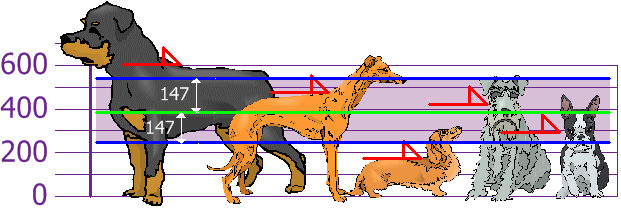
比如现在有5只狗，身高不同，你需要区分或者分类，哪那些是比较高的，那些是比较矮的，怎么界定呢？当然，一眼看上去，哪些高哪些矮还是可以看出来的，但凡事需要有个标准。既然已经提到哪些高矮了，我们可以反过来考虑，为什么不确定哪些为正常身高的呢？一旦确定了正常身高的范围，我们就可以这样分类了：大于这一范围的便是“高的”，小于这一范围的便是“矮的”的。
好了，进入正题，参考上面的图，对于上面的图，我们可以这几只狗的均值和方差（标准差）：
Mean =
$
\mu = \sum{i=1}^m X_i = \frac{600 + 470 + 170 + 430 + 300}{5} = 394
$
Variance
$
\sigma^2 = \frac{1}{m}\sum{i=1}(X_i - \mu)^2 = \frac{206^2 + 76^2 + (−224)^2 + 36^2 + (−94)^2}{5} = 21704
$
Standard Deviation
$
\sigma \approx 147
$
这里，当标准差得到后，我们就可以用其做一些事情了：查看哪些狗位于均值上下一个标准差范围里（$ \mu \pm \sigma$）即：$394 \pm 147$, 位于$[247, 451]$之间的，我们可以将这一部分的身高称作normal的，其他的则为abnormal，比如，高的，矮的，类似下图：

“Rottweilers are tall dogs. And Dachshunds are a bit short”

这里，标准差（standard deviation) 给了我们一准标准方式去区分哪些是normal, 哪些是extra large, 哪些是extra smalle。

Tutorial里还有关于为什么标准差使用平方计算，以及样本和总体的标准差是除以 $n$ 还是 $n-1$ 的讨论。

2: https://www.mathsisfun.com/data/images/statistics-standard-deviation.gif 2019-12-09 18:43:30

期望

$$E(X) = \sum_i^mp_i*x_i$$

如果现在有三个数字1，2，3的转盘，我们估算平均转到的数字是多大？
最自然的想法是求平均，直接(1+2+3)/3 = 2。但如果1,2,3出现的概率不一样呢，比如说:0.5, 0.3, 0.2，那么其均值如何计算？
从合理角度来讲，我们可能需要对每一个出现的数字做一下“加权”：0.51+0.32+0.2*3 = 1.7。
回到上面得到2的结果可以发现，我们默认三个数字出现的概率一样，所以自然而然除以了3，这是基于我们的假设，更或者说我们在未试验之前对系统的一个假设，认为它机会公平。
另外，从上面的表达式可以看出，如果我们手里有一个数据集，比如说6000个样本，要求其期望，我们无需估计每个样本的出现的概率是多少，直接:

$$E(X) = \frac{\sum_i^mx_i}{m}$$

即可，如果样本$x_i$有重复，在sum以及除n的效果下，等效于统计了概率。
换一种说法：如果样本有m个，$x_i$取值有k个(k < m)，根据鸽巢原理，势必会有在每个离散取值的桶里放入了相同元素，垒起来正好是其频次，形似直方图的桶，这样一来再除以总数，正好对应统计上试验得到的频率。

协方差

$$\begin{equation} \begin{array}{l} \operatorname{Cov}(X, Y)=E[(X-E[X])(Y-E[Y])] \\ \operatorname{Cov}(X, Y)=E[X Y]-E[X] E[Y] \end{array} \end{equation}$$

参照上面数据集中期望的算法，可以直接理解为样本的均值，虽然这个均值的实际效果是期望。那么上面