build GPT from scratch
cross_entropy 损失函数估计
1 | class BigramLanguageModel(nn.Module): |
1 | loss = F.cross_entropy(logits, targets) |
其实计算的是
其中:
$p$ 是 softmax 后的概率分布
$y$ 是 ground-truth label (目标token)
$p_y$ 是对应ground-truth 类别的概率
对于这个Loss如果我们想估计一下是什么水平,那就对比随机猜的情况,,这个可以作为baseline
如果模型刚初始化,或者毫无学习能力,其交叉熵损失函数就会非常接近这个值
why loss=4.87 > 4.17 ?
这是因为:模型还没开始训练(刚初始化),预测可能不均匀分布,而是更糟糕的“错误分布”,这会导致预测目标token概率 $p_y \lt fra$
multitorch.multinomial
这个函数用来采样,会根据传入的数据所提供的概率来采样1
2
3
4
5
6
7
8
9
10
11
12
13import torch
# 一维概率分布
probs = torch.tensor([0.2, 0.5, 0.3])
# 采样 3 个样本,不重复采样
samples = torch.multinomial(probs, num_samples=3, replacement=False)
print("Samples:", samples)
# 二维概率分布
probs = torch.tensor([[0.2, 0.5, 0.3], [0.4, 0.4, 0.2]])
# 采样 2 个样本,允许重复采样
samples = torch.multinomial(probs, num_samples=2, replacement=True)
print("Samples:", samples)
temperature
temperature通过在softmax之前修改logits 来平滑或尖锐logits分布
T=1.5:调整后的 logits 更小,概率分布更加平滑,所有类别的概率更加接近。
T=0.5:调整后的 logits 更大,概率分布更加尖锐,最高概率的类别更加突出。1
2
3
4
5
6
7
8
9
10
11
12
13
14
15
16
17
18
19
20
21
22
23import torch
import torch.nn.functional as F
# 定义原始 logits
logits = torch.tensor([[0.1, 0.7, 0.2]])
# 定义温度参数
temperature_high = 1.5
temperature_low = 0.5
# 调整 logits
adjusted_logits_high = logits / temperature_high
adjusted_logits_low = logits / temperature_low
# 转换为概率分布
probs_high = F.softmax(adjusted_logits_high, dim=-1)
probs_low = F.softmax(adjusted_logits_low, dim=-1)
print("Original logits:", logits)
print("Adjusted logits (T=1.5):", adjusted_logits_high)
print("Adjusted logits (T=0.5):", adjusted_logits_low)
print("Probs (T=1.5):", probs_high)
print("Probs (T=0.5):", probs_low)
weighted sum
1 | B, T, C = 2, 4, 2 |
能理解到把x的每一行看做一个2维向量, W每一行对4个2维向量加权求和,如果从矩阵乘法角度去推导,用分块矩阵方式如何具象化这一过程?
关键的地方是只将w分块化,看做行向量的stack, 而x不做分块考虑,这样就直观了.
每一行 output 是对所有 xᵢ(2D 向量)线性加权求和,权重是 W 的一行,这就是 attention 机制里 “加权求和” 的本质。1
2
3
4
5
6
7
8
9
10
11W =
⎡ w₀ᵀ ⎤
⎢ w₁ᵀ ⎥
⎢ w₂ᵀ ⎥
⎣ w₃ᵀ ⎦ ∈ ℝ^{4×4}
W @ x =
⎡ w₀ᵀ @ x ⎤
⎢ w₁ᵀ @ x ⎥
⎢ w₂ᵀ @ x ⎥
⎣ w₃ᵀ @ x ⎦
Query * Key
$\mathrm{res} = \mathrm{Q} \cdot \mathrm{K}^{\top}$ 分块矩阵的理解1
2
3
4
5
6
7
8
9
10
11
12
13
14Q =
---q1---
---q2---
---q3---
K^{T} =
| | |
k1 k2 k3
| | |
res =
[w1, w2, w3]
……
# Q @ K^{T} 是q和K中的emb算sim, 得到weight
attention vs convolution
- Attention is a communication mechanism. Can be seen as nodes in a directed graph looking at each other and aggregating information with a weighted sum from all nodes that point to them, with data-dependent weights.aggregating at each other.
- There is no notion of space. Attention simply acts over a set of vectors. This is why we need to positionally encode tokens.
想象一下transformer里
K, Q, V shape is (B, T, C) = (4, 8, 16)
weight = K @ $\mathrm{Q}^{\mathrm{T}}$ is (B, T, T)
weight @ V = (B, T, C)
没有space 概念,这也是为什么需要add positin embedding的缘故.
虽然通过batch做了并行计算,但从始至终都是每个样本各自independent通信,没有communicate across batch,每个样本是一个有向图结构,各自通信,同一个batch里样本之间所构成的graph是不通信的
- encoder: look all the tokens
- decoder: only look T-1 tokens
self-attention: X -> K, Q, V
cross-attention: X -> K, others-> Q, V
cross attention:
Cross Attention(交叉注意力)是一种注意力机制,常用于需要处理 两个不同输入源之间的交互 的任务中,比如:
图像和文本之间的对齐(如图文生成、视觉问答)
编码器-解码器结构(如机器翻译中的Transformer)
多模态模型(比如 Qwen-VL 这类处理图像+文本输入的模型)
Cross Attention 的核心思想是:
一个序列(称为Query)通过注意力机制来关注另一个序列(称为Key和Value)中的关键信息。
例如:
假设你有一段文本:“这张图片上有什么?”
同时你有一张图片作为输入。
在 cross-attention 中:
文本被当作 Query(提问)
图像特征被当作 Key 和 Value(知识源)
模型会根据文本的每个位置,去图像中找最相关的区域来生成输出
divided by sqrt
“Scaled” attention additional divides wei by 1/sqrt(head_size). This makes it so when input Q,K are unit variance, wei will be unit variance too and Softmax will stay diffuse and not saturate too much. Illustration below1
2
3
4
5
6
7
8
9
10
11
12
13
14
15
16B,T,C = 4,8,32 # batch, time, channels
head_size = 16
k = torch.randn(B,T,head_size)
q = torch.randn(B,T,head_size)
#wei = q @ k.transpose(-2, -1) * head_size**-0.5
wei = q @ k.transpose(-2, -1)
# sqrt version 方差接近1,diffusion
tensor(1.0752)
tensor(0.9134)
tensor(0.9560)
# no sqrt version 方差极端
tensor(0.9716)
tensor(1.0322)
tensor(14.1379)
这样 Softmax 的输出就会比较“分散”(diffuse),而不会“过度饱和”(saturate too much)。
Diffuse” 指 Softmax 输出的分布比较“均匀”,不会只有几个值接近 1,其它都是 0。
“Saturate” 是指当输入非常大或非常小,Softmax 的输出趋近于极值(0 或 1),梯度会消失或训练不稳定。
如果没有 scale(√d),Q·K 的 dot product 会随 head_size 增大而变大 → 造成 Softmax 输出饱和 → 注意力只盯住很少几个 token → 学不到全局信息。
数学解释
$\mathrm{Var}(QK) = \mathrm{E}[(QK)^2] - (\mathrm{E}[QK])^2 = 1-0 = 1$
因为Q, K 相互独立,所Q, K的联合概率密度可以表示为他们的边缘概率分布乘积(平方也是)
it means:
$\mathrm{E}[QK] = \mathrm{E}[Q]\cdot\mathrm{E}[K]$
那么
所以这是后除以$\sqrt{d_k}$会使得方差恒定,不会变化非常大
register_buffer
一些不需要train的变量可以注册为buffer, 例如统计量mean, std, mask
Transformer
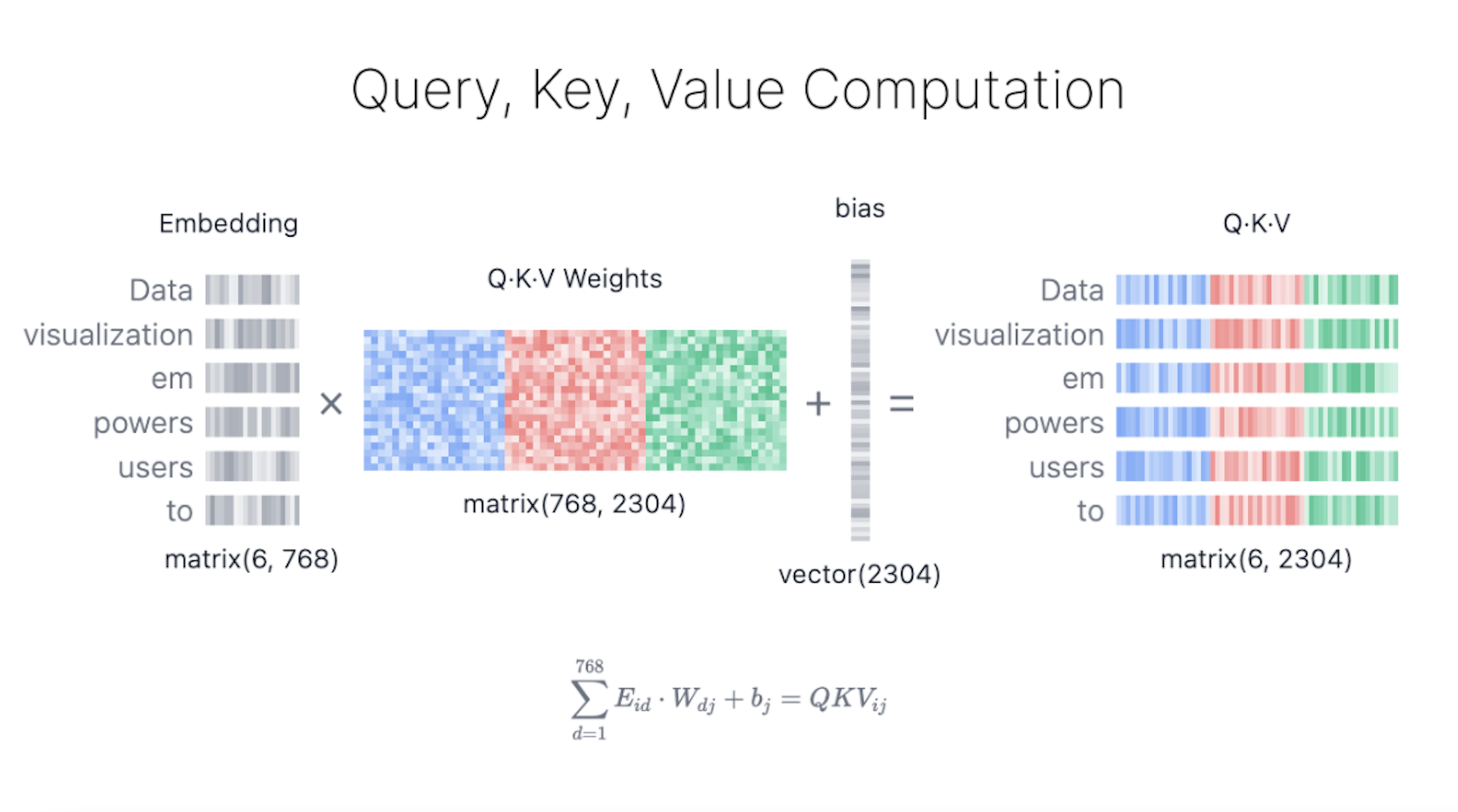
Query, Key, and Value Matrics
Q, K, V 的生成式并行化的,通过把Weight stack在一起,通过一次矩阵乘法得到1
(T, C) @ (C, C*3) -> (T, C*3)
here T = 6, C = 768